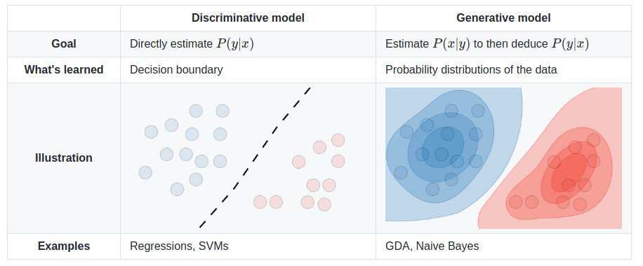
The SVM algorithm classifies data points into categories by finding a boundry between groups that leaves the largest possible gap. Where the boundry is clear, but the data is distributed, Logistic Regression may be less costly. SVMs can efficiently perform non-linear classification and commonly uses the kernal trick which provides training features related to the distance of each data point from the others. Highly optimized librarys of code are available to implement SVMs such as liblinear^ or libsvm^. This is a discriminative model which directly predicts the output class division rather than look at the distribution of the classes. It works best where the data is not clustered, but has a clear boundry. Unlike regression, SVM will find the best possible boundry, centered between the data. When the data is grouped in obvious clusters, Naive Bayes may work better.

  Logistic Regression Cost
|
SVM is very similar to Logistic Regression. The major difference is that in order to more easily support the Kernel trick described below, the cost function for SVM has been changed as follows:
• Instead of using lambda to scale the weight of the theta parameters for regularization, we use "C" to scale the weight of the main part of the cost function. So, where a large lambda would penalize parameters, now a small C does the same; leaving the parameters large while the rest of the function becomes small.
• The regularization term, can then be written as
OTO if we exclude
O0. Some implmentations use a different transform
for regularization inorder to further reduce computational cost.
• Because we don't need to worry about derivatives in the same way, we can remove the division by m. Since m is a constant, the cost function will still help us converge on the same minimum.
 •
Instead of using the sigmoid function, we replace that with two separate
cost functions, cost0 and cost1. They produce a graph
very much like the sigmoid, but with straight lines instead of a curve.
• The cost0 and cost1 functions are more selective because we set the
boundary at 1 and -1 instead of at 0. E.g. We look for
OTx(i) >= 1 if
y(i) = 1
OTx(i) <= -1 if
y(i) = 0
Because of this "no mans land" or overlap between the costs, given
regularization to find the smallist possible
values of O (theta), SVM not only finds a boundary, it finds
the boundary that puts the most distance between it and the training examples.
Note: Many SVM implementation already support multiple classes, but to add
that support, you can simply train multiple SVMs, each recognizing only one
class, then pick the class with the highest confidence; the highest
OTx(i).
• Instead of features based directly on the data, we use Kernel features that describe the distance from each data point.
Kernals compute the simularity between a "landmark" and any given training example.
One common type of Kernel is the Gaussian or RBF Kernel^ or exp( -||x - l(i)||2 / 2Ó2 ). The ||x - l(i)|| part is the distance between the landmark and the example. When they are close, the result is close to 1. When they are distant, it will be close to 0. The value of Ó controls how sharply the comparison "falls off". e.g. with a large Ó being anywhere near the landmark will register with that feature. With a small Ó, as soon as the point moves away from the landmark, the feature quickly drops out.
Each of the landmarks can be used to make a new feature for the polynomial. Using this feature would allow the system to learn if the outcome is related to the data point being "close" to this landmark. While training, we can place landmarks at each training example, so there are m landmarks i.e. one feature for each data point in the training set, instead of one feature for each dimension of those points. The resulting features can replace the original features from the training data because one of them will be 0 distance from each data point. The means the polynomale features are comparing the distances between the data points. When points in one class are near each other, those features develop higher theta parameters. Computational cost is related to training set size, not to the dimensions of each data point. In the regularization part of the cost formula, n will equal m.
In Octave a possible Gaussian Kernal is:
function sim = gaussianKernel(x1, x2, sigma)
	x1 = x1(:); x2 = x2(:); %make column vectors
	sim = exp(sum((x1-x2).^2) / (-2 * sigma.^2));
	end
svmtrain (from SVMLIB as installed^ in Octave for example) takes training data X and y, and some value for C and sigma, then returns a model :
libsvm_options = ' '-c 1 -g 0.07 -b 1'; %-b only reqired for confidence
model = svmtrain(y, X, libsvm_options);
[predict, accuracy, confidence]  = svmpredict(yval, Xval, model);
%yval is required but can be random if accuracy is not required
%Xval is the validation set
% see https://github.com/cjlin1/libsvm/tree/master/matlab for more
Note: Use feature scaling if using the Gaussian Kernel.
Note: Only use similarity functions that satisfy "Mercer's Theorem"^. There are many such functions, including: Polynomia, String, Chi-squared, Histogram, Intersection
An SVM can be made with no Kernel (this is sometimes called a "linear kernel") This works well, and can avoid overfitting, for a large number of features and small sample set. (n > m) or for a very large sample set ( m > 50,000 ) although Logistic Regression may be a better choice.
The Gaussian Kernel SVM is best for small feature sets ( n < 1000 ) and reasonable sample sets ( 10 < m < 10,000 ). Within this range, it can work as well as a Neural Net and avoid the slow back propigation training.
In Python using svm.SVC from SciKit-Learn.org:
import sys
from time import time
import numpy
from sklearn.svm import SVC

### Load features_train, labels_train as numpy arrays of features and lables.
### Make features_test, labels_test as subsets of the training data for testing.

classifier = SVC(kernel='rbf',C=10000)
### kernal could be linear, polynomial, rbf, or sigmoid

t0 = time()
fit = classifier.fit(features_train, labels_train)
print "training time:", round(time()-t0, 3), "s"

t0 = time()
prediction = classifier.predict(features_test)
print "prediction time:", round(time()-t0, 3), "s"
print prediction

score = classifier.score(features_test,labels_test)
print score
See also:
| file: /Techref/method/ai/SupportVectorMachine.htm, 9KB, , updated: 2019/3/6 11:28, local time: 2025/9/27 15:02,
owner: JMN-EFP-786,
216.73.216.85,10-1-214-182:LOG IN
|
| ©2025 These pages are served without commercial sponsorship. (No popup ads, etc...).Bandwidth abuse increases hosting cost forcing sponsorship or shutdown. This server aggressively defends against automated copying for any reason including offline viewing, duplication, etc... Please respect this requirement and DO NOT RIP THIS SITE. Questions? <A HREF="http://massmind.org/Techref/method/ai/SupportVectorMachine.htm"> Support Vector Machine</A> |
| Did you find what you needed? |
Welcome to massmind.org! |
Welcome to massmind.org! |
.