Stepping Motion Profiles in Realtime
by VegiPete copied with permission from http://picprog.strongedge.net/step_prof/step-profile.html
- This page describes the needs of motion profiles and presents an algorithm for generating these profiles in real time using a PIC18F series microcontroller.
Overview
-
Stepping motors are a commonly used item for generating controlled motion. (Wikipedia can be reviewed for a more expansive description of stepper motors.) Typical stepper motor controllers require simple step and direction signals to move a stepper motor. (LiniStepper and GeckoDrive are two examples of stepper controllers.) Furthermore, some servomotor controllers (for example, Granite Devices and Viper) also understand step and direction signals. It is the job of the motion controller to generate the sequence of step pulses and direction signals that result in the motor moving smoothly and accurately to the desired position and/or velocity.

-
Figure 1: Basic Components of a Simple Motion Control System
The basic parts required for simple motion control are shown in figure 1. Usually a power supply is also required.
-
Motion Controller: the component that generates the sequence of step and direction signals required to move the motor in the desired way. In the case of CNC machine tools, this is often a PC running software such as EMC or MACH, generally sending signals by means of a parallel printer port, usually controlling multiple drives and motors. PLCs or microcontrollers can be used for simpler tasks.
-
Motor Controller or Driver: the component that interprets step and direction signals and converts and amplifies them into (usually) higher power currents that actually drive the motor. Handles phase sequencing, current levels and other aspects of driving the connected motor.
-
Motor: the actuator that receives electrical impulses and converts them to mechanical motion.
- Power Supply: provides the motivated electrons than are use to generate the magnetic fields within the motor. Often a separate power supply provides clean power to the control electronics.
An important issue with stepper motors is that they are usually used in an open loop. This means that the motor control system has no feed back about motor position. The system requests that the motor move but cannot determine if the motor actually did move as commanded. If the mechanical system has been designed correctly and is operating as it should without overloads, the motor can be expected to move as desired. (This contrasts with a servo system which does have feed back and hence knows that the motor is moving as demanded. Also, a more advanced stepper system could be implemented with position feed back.)
-
Some Physics of Motion
-
One of the most basic equations of motion is
-
-
- F = ma
-
In words, this equation explains that force is equal to mass times acceleration. This equation is very relevant to stepper motor motion because it relates the force needed to accelerate the mechanical system to the mass of the system. (Actually the inertia of the system if you want to be picky.) If a stepper motor can only generate a certain amount of force, the system mass will determine the maximum acceleration. Attempting to accelerate faster will result in an overload and the likely loss of steps. As long as the acceleration is kept safely below this maximum, the mechanical system can be expected to faithfully follow the requested steps.

-
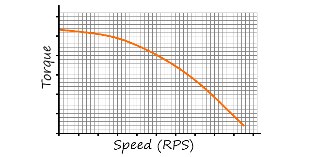
Figure 2: Typical Torque Curve of a Stepper Motor
The other important physics characteristic that must be mentioned is the maximum velocity. Motors have what is known as a torque curve. The general characteristic of these curves is that motor torque falls off as the speed increases, as shown in figure 2. Thus, at higher speeds, a motor generates less force. The actual shape of the curve depends on the details of the motor and its driver. This results in a maximum effective speed above which the mechanical system could start to skip or loose steps.
-
The Shape of a Move
-
Now we know enough to consider how to actually perform a desired move. The
size of the move is given as a particular number of steps. We know that there
is a maximum allowable speed, the maximum steps per second. The motor will
be stopped before the move starts and after the move is completed. We know
that the motor cannot go from stationary to maximum speed instantly, nor
can it stop instantly. Instead, speed changes are limited by the maximum
allowable acceleration.

-
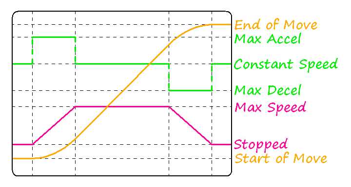
Figure 3: Distance, Velocity and Acceleration During a Trapezoidal Move
We can plot a graph of distance, speed and acceleration over the duration of a move, as shown in figure 3. This particular motion profile has been chosen with only maximum acceleration and deceleration, resulting in a so called trapezoidal speed profile. Two characteristics of this particular profile are linear speed changes and equal acceleration and deceleration periods. These characteristics are useful because they simplify the calculations required during the move. For shorter moves, the maximum speed will not be reached before the mid-point of the move. In that case, deceleration will begin at the mid-point, cutting out the constant speed centre section and resulting in a triangular speed profile.
-
A Sequence of Steps
-
We can now consider the actual sequence of steps that will result in the
motor turning as required. These steps will appear as pulses on the STEP
data line with the DIRECTION data line set HI or LOW depending on the required
direction.

-
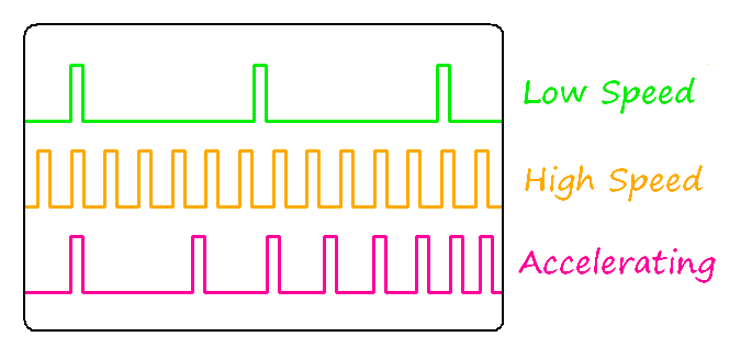
Figure 4: Constant Speed and Accelerating Step Sequences
These step sequences, known as pulse trains, must be generated by the motion controller. Pulses for constant speed are easy to generate - the time between each pulse is the same. The acceleration and deceleration pulses trains are more difficult to generate because the time between pulses varies in a non-linear way. Accurate timing requires the calculation of reciprocals or square roots in real time, which can require more mathematical computation than is available from a low power microcontroller.
Various algorithms have been developed to simplify these computations at the cost of some loss of accuracy. The primary paper seems to be D. Austin's "Generate stepper-motor speed profiles in real time." (The source code is available here.) The AVR world also has an app note and source code based on D. Austin's paper. A chief characteristic of this algorithm is that it computes time per step .
Alternate techniques use precomputed data tables but that obviously removes the on-the-fly adjustability of real time pulse train generation.
A different algorithm is presented by Pramod Ranade in his article Linear motor control without the math. His method in effect computes steps per time , the reciprocal of the D. Austin's method above. This change simplifies the computations significantly. The source code associated with this article so far remains elusive so P. Ramade's implementation is unknown. The remainder of this page describes my implementation of this steps per time algorithm.
-
Steps per Time instead of Time per Step
-
At its heart, the Steps per Time algorithm (SpTA) divides time into
a suitably small unit and checks at each time unit whether it is time to
generate a new step pulse. This is actually implemented by adding a fraction
of a step to the current position at each time period and then only generating
a step pulse if the position fraction overflows. The fraction of a step that
is added is actually the speed, which can itself be adjusted by the acceleration
at each time unit to give constant acceleration speed ramps. P. Ranade's
paper linked above gives a more complete example.
My implementation uses a timer interrupt to create the fixed time units and a number of multi-byte variables to hold the various values. The algorithm relies only on additions and comparisons to perform a move, with a single divide-by-two operation, a simple right shift, at the start to compute the mid-point of the move. With a PIC18F series microcontroller at 10 MIPS, I have managed to comfortably generate step pulses at 60kHz.
Let's have a look at how the code works.
A state machine is used to track the required conditions during a move profile. The 4 required states are
-
0: Idle - no move currently active
1: Decelerating - approaching end of move
2: At_Max - moving at full speed
3: Accelerating - move starting
To start, here is some pseudo-code that represents the required computation. This pseudo-code would be executed for each time period - in other words, each time the periodic timer interrupt occurs.
-
/* Calculate next time slice, generate step pulse if needed */
step_count_fraction = step_count_fraction + present_speed
IF Carry THEN
	step_count = step_count + 1
	generate step output pulse

/* Adjust stepping speed if needed, depending on state */
IF state = Accelerating THEN
	present_speed = present_speed + acceleration
	IF step_count = midpoint THEN
		set state = Decelerating
		done
	IF present_speed >= max_speed THEN
		calculate deceleration_start
		set state = At_Max
	done
IF state = At_Max AND step_count = deceleration_start THEN
	set state = Decelerating
	done
IF state = Decelerating THEN
	present_speed = present_speed - acceleration
	If step_count = total_move_count THEN
		set state = Idle
done
Most of this is quite straight forward. Perhaps the only tricky part is that two different events can cause the acceleration state to end. If the mid-point of the move is reached while still accelerating, it's time to start decelerating because this profile will be a triangle profile. If the maximum speed is reached, a full trapezoidal profile is called for and the start point for deceleration must be calculated. Since the acceleration and deceleration rates are the same, the number of steps during these states will be the same. This allows the start of the deceleration state to be calculated as the total number of steps requested minus the number of steps taken during the acceleration state.
Here are the main variables used by the code:
-
;step ramp control variables
;the first 3 variables should be set by the calling routine
;(the direction line must also be set by the calling routine)
;the other vars will be handled by the call to Start_Move
CBLOCK
step_move:4     ;total move requested
step_spmax:2    ;maximum speed
step_accel:2    ;accel/decel rate, 8.8 bit format

step_middle:4   ;mid-point of move, = (step_move - 1) >> 1
step_count:4    ;step counter
step_frac:2     ;step counter fraction
step_speed:4    ;current speed, 16.8 bit format (HI byte always 0)
step_state:1    ;move profile state
step_dur:1      ;counter for duration of step pulse HI
ENDC
Most of these variables represent multi-byte fixed point values. These fixed point values align as follows:
-
step_count

(32.0 bits) step_frac

(0.16 bits) step_speed

(16.8 bits - highest byte is always 0) step_accel

(8.8 bits)
The source code is available in the Stepper Speed Ramps forum^.
Send any comments, concerns, questions or anything else to vegipete at this domain dot net. -